Simpson’s paradox
Often when one mentions “a relationship between variables” we think of a relationship between just two variables, say a so called explanatory variable, \(x\), and response variable, \(y\). However, truly understanding the relationship between two variables might require considering other potentially related variables as well, often referred to as confounding variables. If we don’t, we might find ourselves in a Simpson’s paradox. So, what is Simpson’s paradox?
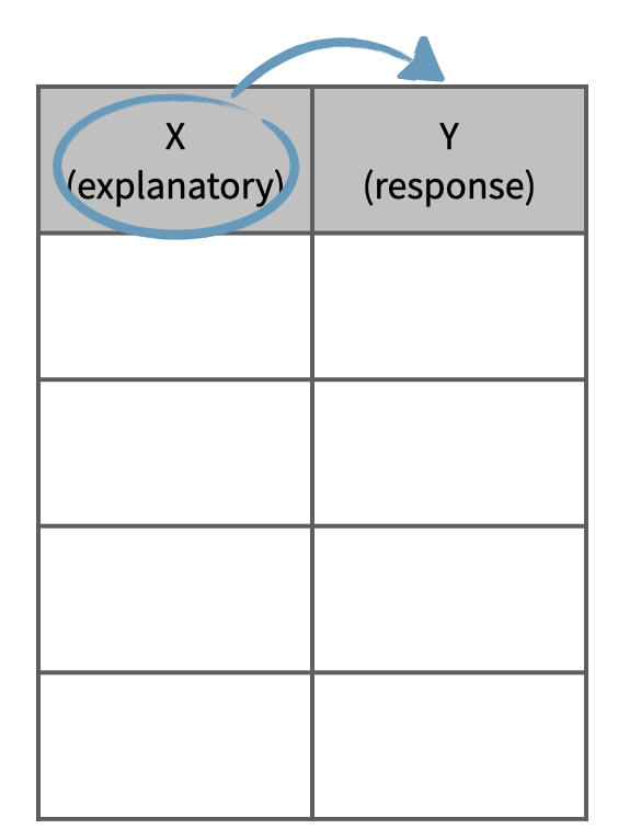
First, let’s clarify what we mean when we say explanatory and response variables. Labeling variables as explanatory and response does not guarantee the relationship between the two is actually causal, even if there is an association identified. We use these labels only to keep track of which variable we suspect affects the other.
Explanatory and response
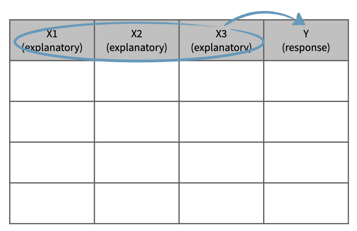
And these definitions can be expanded to more than just two variables. For example, we could study the relationship between three explanatory variables and a single response variable.
Multivariate relationships & confounding
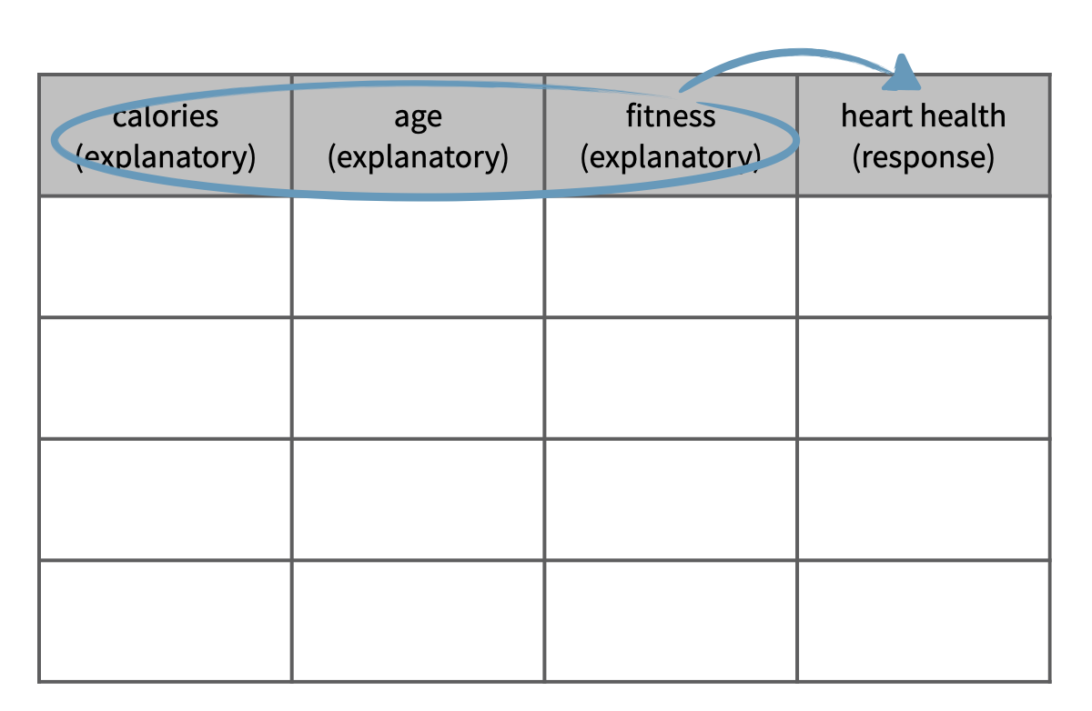
This is often a more realistic scenario since most real world relationships are multivariable. For example, if we’re interested in the relationship between calories consumed daily and heart health, we would probably also want to consider information on variables like age and fitness level of the person as well.
In statistical terms, age and fitness level are potential confounders in the relationship between calories consumed and heart health. You’ll talk about confounders in more detail in others classes, but just know that a confounding variable is a factor that is associated both with the response and the explanatory variable or interest. A confounding variable may distort or mask the effects of another variable on the disease in question and always needs to be considered in an analysis.
Not considering an important variable when studying a relationship can result, in extreme cases, in what we call Simpson’s paradox. This paradox illustrates the effect the omission of an explanatory variable can have on the measure of association between another explanatory variable and the response variable. In other words, the inclusion of a third variable in the analysis can change the apparent relationship between the other two variables.
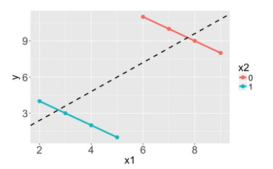
Consider the eight dots in the scatter plot below (the points happen to fall on the orange and blue lines). The trend describing the points when only considering x1 and y, illustrated by the black dashed line, is reversed when x2, the grouping variable, is also considered. If we don’t consider x2, the relationship between x1 and y is positive. If we do consider x2, we see that within each group the relationship between x1 and y is actually negative.
We’ll explore Simpson’s paradox further with another dataset, which comes from a study carried out by the graduate Division of the University of California, Berkeley in the early 70’s to evaluate whether there was a sex bias in graduate admissions. The data come from six departments. For confidentiality we’ll call them A through F. The dataset contains information on whether the applicant identified as male or female, recorded as Gender, and whether they were admitted or rejected, recorded as Admit. First, we will evaluate whether the percentage of males admitted is indeed higher than females, overall. Next, we will calculate the same percentage for each individual department.
Berkeley admission data
| Admitted | Rejected | |
|---|---|---|
| Male | 1198 | 1493 |
| Female | 557 | 1278 |
Note: At the time of this study, gender and sexual identities were not given distinct names. Instead, it was common for a survey to ask for your “gender” and then provide you with the options of “male” and “female.” Today, we better understand how an individual’s gender and sexual identities are different pieces of who they are. To learn more about inclusive language surrounding gender and sexual identities see the gender unicorn.
Let’s get started.
Number of males and females admitted
The goal of this exercise is to determine the numbers and proportions of male and female applicants who got admitted and rejected. Specifically, we want to find out how many males are admitted and how many are rejected. And similarly we want to find how many females are admitted and how many are rejected.
Let’s first load and check the ucb_admit dataset:
* Initialize SAS workspace;
%include "~/my_shared_file_links/hammi002/sasprog/run_first.sas";

* Makes a working copy of UCB_ADMIT data and glimpse;
%use_data(ucb_admit);
%glimpse(ucb_admit);
To count admissions and see admission rates by group, we will use PROC FREQ:
* Count admissions by male/female;
proc freq data=ucb_admit;
	tables gender * admitted / nocol nopct;
run;
The nocol and nopct options above suppress the column and overall percentages from being shown, so we are left with just the counts and the row percentages (i.e., % of each group that is admitted). This is what we’re after since the first variable (gender) in a 2-variable tables statement defines the row variable, while the second variable (admitted) defines the column variable.
Based on the resulting table, answer the following question: Which gender had a higher admission rate, male or female?
Proportion of males admitted for each department
Finally we’ll make a table similar to the one we constructed earlier, except we’ll first group the data by department. The goal is to compare the proportions of male students admitted across departments.
We can do this easily by adding a third variable in the PROC FREQ tables statement, prior to the variable that are there already, as:
* Count admissions by male/female, by department;
proc freq data=ucb_admit;
	tables dept * gender * admitted / nocol nopct;
run;
Now the percentages shown reflect the male/female-specific admission rates separately for each department.
Based on these results, which of the following statements best describes the relationship between admission status and gender?
- Within most departments, female applicants are more likely to be admitted.
- Within most departments, male applicants are more likely to be admitted.
- Within most departments, male and female applicants are equally likely to be admitted.
Surprising given the overall results, no?
Recap: Simpson’s paradox
We’ll wrap up the lesson with a recap of our findings.
Overall, males were more likely to be admitted. Within most department, however, females were more likely to be admitted. Meaning, when controlling for department, the relationship between gender and admission status was reversed. This is Simpson’s paradox.
We would have to know about the data to tease out the reasons for this, but one potential explanation for this paradox is that women tended to apply to competitive departments with lower rates of admission even among qualified applicants, such as in the English Department. Whereas, men tended to apply to less competitive departments with higher rates of admission among the qualified applicants, such as in engineering and chemistry.
Note that we were only able to discover the contradictory finding once we incorporated information about the department of the application. Examples like this highlight the importance of a good study design that considers and collects information on extraneous, but potentially confounding variables in a study.
You have successfully completed this tutorial.