Inference for one mean

Let’s move on to talking about inference for numerical variables. The most common population parameter of interest for numerical variables is the mean. And, as we did with proportions, we’ll walk through both the randomization methods and the mathematical methods for inference.

For this lesson, we’ll use information about births in North Carolina. Actually, we’re going to take a look at the mothers’ weight gain during pregnancy. Let’s load the data and ignore any records with missing information on that variable. Let’s also load the randomization macros.

* Initialize this SAS session;
%include "~/my_shared_file_links/hammi002/sasprog/run_first.sas";

* Load randomization macros;
%include "~/my_shared_file_links/hammi002/sasprog/load-randomization.sas";

* Makes a working copy of NCBIRTHS data and check;
%use_data(ncbirths);
%glimpse(ncbirths);

* Remove observations with missing information about weight gain;
data ncbirths;
	set ncbirths(
		where=(not missing(gained))
	);
run;

Before we start the inference procedures, let’ s calculate mean weight gain and take a look at the observed distribution:

* Summarize weight gain information;
proc means data=ncbirths mean std median q1 q3 maxdec=1;
	var gained;
run;

* Histogram of weight gain;
proc sgplot data=ncbirths;
	histogram gained;
run;

Mean (SD) weight gain was 30.3 (14.2) pounds. And, from the histogram, we can see that the range was 0 pounds to over 80 pounds.

Bootstrapping for confidence intervals

Bootstrapping for hypothesis testing

Before talking about the mathematical model for inference for one mean, let’s briefly talk about the randomization methods that we would use.

Re-centering a bootstrap distribution

So far we learned how to create bootstrap confidence intervals for estimation purposes. But what do we do if our goal is testing, not estimation? How can we use simulation methods to test whether a single parameter of a numerical distribution is different from, greater than, or smaller than some value? The answer is simple, though not necessarily intuitive. However if you keep in mind one important aspect of hypothesis testing – namely that we assume the null hypothesis is true – hopefully the approach makes sense.

Re-centering a bootstrap distribution for hypothesis testing

• Bootstrap distributions are by design centered at the observed sample statistic.
• However since in a hypothesis test we assume that $H_0$ is true, we shift the bootstrap distribution to be centered at the null value.
• p-value = The proportion of simulations that yield a sample statistic at least as favorable to the alternative hypothesis as the observed sample statistic.

Bootstrap distributions are by design centered at the observed sample statistic.

However since in a hypothesis test we assume that the null hypothesis is true, we shift the bootstrap distribution to be centered at the null value.

The p-value is then defined as the proportion of simulations that yield a sample statistic at least as favorable to the alternative hypothesis as the observed sample statistic.

Re-centering the bootstrap distribution - sketch

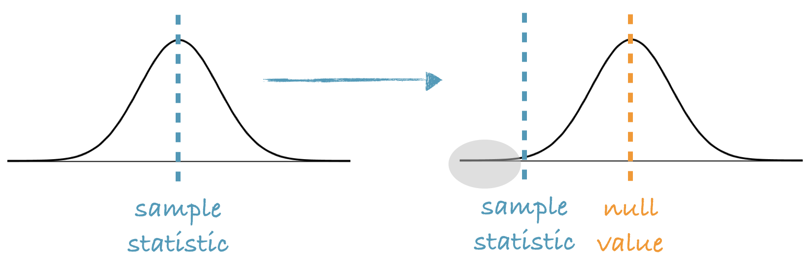
Here is a graphical representation: We start with our bootstrap distribution, which is always centered at the observed sample statistic. We then shift this distribution so the center is at the null value, and calculate the p-value as the proportion of simulations that yield bootstrap statistics that are at least as extreme as the observed sample statistic.