Inference for one mean
Let’s move on to talking about inference for numerical variables. The most common population parameter of interest for numerical variables is the mean. And, as we did with proportions, we’ll walk through both the randomization methods and the mathematical methods for inference.
For this lesson, we’ll use information about births in North Carolina. Actually, we’re going to take a look at the mothers’ weight gain during pregnancy. Let’s load the data and ignore any records with missing information on that variable. Let’s also load the randomization macros.
* Initialize this SAS session;
%include "~/my_shared_file_links/hammi002/sasprog/run_first.sas";

* Load randomization macros;
%include "~/my_shared_file_links/hammi002/sasprog/load-randomization.sas";

* Makes a working copy of NCBIRTHS data and check;
%use_data(ncbirths);
%glimpse(ncbirths);

* Remove observations with missing information about weight gain;
data ncbirths;
	set ncbirths(
		where=(not missing(gained))
	);
run;
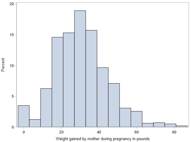
Before we start the inference procedures, let’ s calculate mean weight gain and take a look at the observed distribution:
* Summarize weight gain information;
proc means data=ncbirths n mean std median q1 q3 maxdec=2;
	var gained;
run;

* Histogram of weight gain;
proc sgplot data=ncbirths;
	histogram gained;
run;
Among these 973 mothers, mean (SD) weight gain was 30.3 (14.2) pounds. And, from the histogram, we can see that the range was 0 pounds to over 80 pounds.
Bootstrapping for confidence intervals
Before talking about the mathematical model for inference for one mean, let’s briefly talk about the randomization methods that we would use.
If we wanted an assumption-free way to get a 95% confidence interval around our observed mean of 30.3, we can always use bootstrapping and calculate a confidence interval using either the bootstrap standard error method or the bootstrap percentile method. For simplicity, let’s just use the latter, based on 10,000 bootstrap re-samples.
* Bootstrap confidence interval, single mean, 10000 samples;
%boot_1mean(
	ds = ncbirths,
	dovar = gained,
	alpha = 0.05,
	reps = 10000
);
What is the interval you get? Mine was (29.4, 31.2) pounds. Meaning (always interpret!) that, with 95% confidence, we expect the true mean weight gain among mothers in North Carolina to be between 29.4 and 31.2 pounds.
As a knowledge check, how would you calculate a confidence interval using the bootstrap standard error that is also output by this macro?
Bootstrapping for hypothesis testing
We may also want to test our single mean value against a specific null value. When we were dealing with proportions, we just simulated the null distribution by creating samples from a hypothetical population with a known (null) distribution of the characteristic of interest. That was possible because, essentially, flipping a coin (or a biased coin, as needed for a proportion not equal to 0.5) is all that is needed to create that hypothetical population.
With numerical data, if we want to create a hypothetical population with a specific mean value, we also must know the variability of those values within the population (typically measured by the standard deviation), which is not something we typically know. But, if we treat our sample as a representation of the source population, we can use the variability of our observed data to estimate the true variability in this source population.
And what we just described was the bootstrapping methodology, with one twist. Because bootstrap distributions are, by design, centered at the observed sample statistic, this distribution won’t work as a null distribution against which we can compare our observed statistic.
However since in a hypothesis test we assume that \(H_0\) is true, we can shift, or re-center, the bootstrap distribution to be centered at the required null value, then, as with other randomization tests, calculate the p-value as the proportion of bootstrap samples that yield a sample statistic at least as extreme as the observed sample statistic.
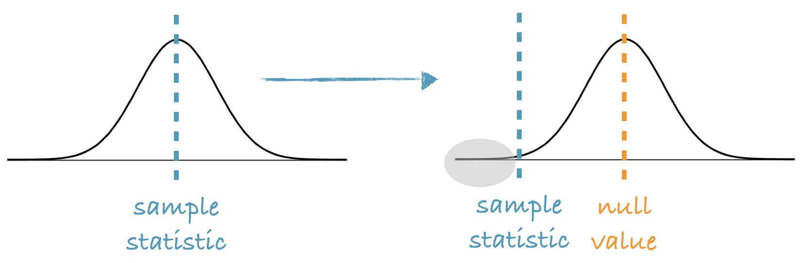
Here is a graphical representation: We start with our bootstrap distribution, which is always centered at the observed sample statistic. We then shift this distribution so the center is at the null value, and calculate the p-value as the proportion of simulations that yield bootstrap statistics that are at least as extreme as the observed sample statistic.
This isn’t something you’ll need to do manually, however. It’s all handled in the SAS macro for a single mean. Let’s run an example.
Suppose a researcher in South Carolina has use their birth data to estimate that mothers in South Carolina gain, on average 31.1 pounds during pregnancy. You are interested to know if weight gain during pregnancy in North Carolina is different.
In this instance, we only have 1 parameter of interest, the mean weight gain during pregnancy of NC mothers, \(\mu_{NC}\). (The value in SC is given. We don’t have any data from SC.) And the research hypotheses would be:
- \(H_0: \mu_{NC} = 31.1\) pounds
- \(H_A: \mu_{NC} \neq 31.1\) pounds
Let’s use \(\alpha = 0.05\), since a significance level was not specified. We know our observed statistic is 30.3 pounds, but now need to use the shifted bootstrap to test.
* Hypothesis testing, single mean, 10000 samples;
%test_1mean(
	ds = ncbirths,
	dovar = gained,
	nullval = 31.1,
	reps = 10000
);
If we look at the histogram of the null distribution that is output, we can see that it is centered not at the sample statistic (30.3), but at the null hypothesized value (31.1). That is because of the re-centering that is needed to make this a null distribution. (As a reminder, the solid red line represents our observed value and the dotted red line represents the value that is as far from the null in the other direction.)
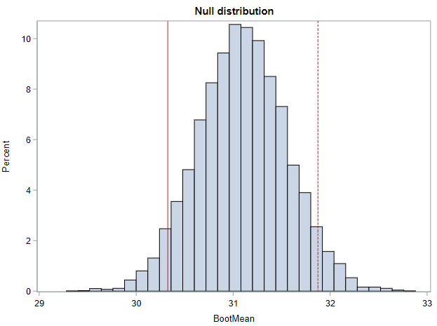
Based on the output, the 2-sided p-value from this randomization test (for me) is 0.090. At \(\alpha = 0.05\), our result is not statistically significant and we cannot reject the null hypothesis. We do not have enough evidence to conclude that mean weight gain in NC is different from mean weight gain in SC.
Now let’s move to the mathematical model.
Mathematical approximation using the t-distribution
When the parameter of interest is the mean (or a difference between two means) and certain conditions are not violated, we can also use methods based on the Central Limit Theorem for conducting inference.
Unfortunately, as the book notes, in order to use the normal distribution as a good approximation for our sample mean, based on the Central Limit Theorem, we must know the true population \(\sigma\), which is almost always unknown to us. And when we use the sample standard deviation, \(s\), as an estimate of \(\sigma\), the normal approximation is no longer perfect. But the related t-distribution is able to act as a suitable mathematical approximation.
In a nutshell the t-distribution is useful for describing the distribution of the sample mean when the population standard deviation, \(\sigma\), is unknown, which is almost always.
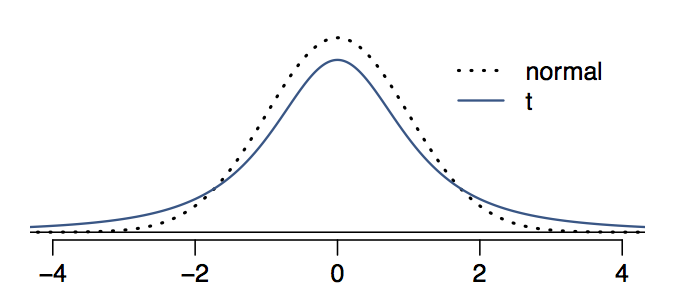
This distribution also has a bell shape, so it’s unimodal and symmetric. It looks a lot like the normal distribution, however its tails are thicker.
Comparing the normal and t distributions visually is the best way to understand what we mean by “thick tails”. Notice that the peak of the t-distribution doesn’t go as high as the peak of the normal distribution. In other words, the t-distribution is somewhat squished in the middle, and the additional area is added to the tails.
This means that, under the t-distribution, observations are more likely to fall 2 SD away from the mean than under the normal distribution. This implies that confidence intervals constructed using the t-distribution will be slightly wider (i.e., more conservative) than those constructed with the normal distribution.
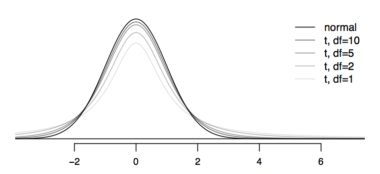
Like the standard normal z-distribution, the t-distribution is always centered at zero. Unlike the z, however, it has one parameter, degrees of freedom, which determines the thickness of its tails. We’ve seen degrees of freedom before, with the chi-square distribution. So, like the chi-square distribution, the t-distribution is not a single distribution, but series of distributions, depending on the df of the data.
In general, when working with means, \(df = n - 1\).
What happens to the shape of the t-distribution as the degrees of freedom (i.e., sample size) increases?
The plot above shows a series of bell curves, going from light to dark shades of gray as the degrees of freedom increases.
We can see that as the degrees of freedom increases, the t-distribution approaches the normal distribution.
This is why you might see in other resources that if the sample size is “large enough”, one can use the normal distribution to approximate the sampling distribution of the mean. Often such statements will be accompanied by a sample size that can be considered “large enough” for the statement to hold. In this tutorial, we will keep things straightforward—when working with the mean (or difference of means), we will use the t-distribution for Central Limit Theorem-based inference.
Probabilities under the t-distribution
If you look at the Excel p-value workbook, you’ll see there is a section for the t-distribution. Pull up that workbook to have some practice getting probabilities associated with the t-distribution.
- Find the probability, under the t-distribution with 10 degrees of freedom, of a t-value less than 3.0, \(P(t < 3.0) =\) ?
- Find the probability, under the t-distribution with 10 degrees of freedom, of a t-value with magnitude greater than 2.0 (i.e., two-tailed), \(P(abs(t) > 2.0) =\) ?
- Find the probability, under the t-distribution with 100 degrees of freedom, of a t-value with magnitude greater than 2.0 (i.e., two-tailed), \(P(abs(t) > 2.0) =\) ?
- How do the last two probabilities compare? Why?
Cutoffs under the t-distribution
We can also use the Excel workbook to get critical values (cutoffs) under the t-distribution associated with specific significance levels, \(\alpha\). For a given \(\alpha\) and a given degrees of freedom, \(df\), the critical value, \(t^*\), is the value of the t-distribution for which the probability of more extreme values, in one or both tails, is \(100\alpha\)%.
Again, use the workbook to practice getting critical values associated with the t-distribution.
- Find the critical value, \(t^*\) for \(\alpha = 0.01\) under a t-distribution with 10 degrees of freedom.
- Find the critical value, \(t^*\) for \(\alpha = 0.05\) under a t-distribution with 10 degrees of freedom.
- Find the critical value, \(t^*\) for \(\alpha = 0.05\) under a t-distribution with 100 degrees of freedom.
- How do the last critical values compare? Which is closer to the normal based critical value of 1.96 for an \(\alpha = 0.05\)?
Assumptions required for the t-distribution
In order to be able to rely on the t-distribution as a suitable approximation, our data must meet the following two assumptions:
- The sample observations must be independent. As we have discussed before, you assess this assumption based on your knowledge of sampling design and measurement methodology.
- The underlying data must be normally distributed. When n < 30, we are generally OK assuming the underlying data are normally distributed if there are not clear outliers. When n is 30 or larger, we are almost always OK assuming the underlying data are normally distributed. Any outliers with a larger sample size must be truly extreme to make this approximation unsuitable.
The NC birth data we are using as an example easily meets both of these criteria.
Confidence intervals with the t-distribution
In order to use the t-distribution as our mathematical approximation for calculating a confidence interval, we need to adjust our formula:
\[CI = SampleStatistic \pm t^{*}_{df} \times SE\]We already know our sample statistic. The mean weight gain in our population was 30.3 pounds. We just need \(t^*\) and the standard error.
We talked above about how to get an appropriate \(t^*\) critical value. Let find that critical value for our data, with 973 observations, using a significance level, \(\alpha = 0.05\). First, we calculate our degrees of freedom, \(df = n - 1 = 973 - 1 = 972\). Now, we use Excel workbook to find that \(t^{*}_{972} = 1.96\). This should look familiar. Given enough sample size, the t-distribution truly does resemble the standard normal distribution.
The standard error associated with a mean, based on sample’s observed variability is:
\[SE = s / \sqrt{n}\]For our data, using the SD we calculated at the beginning of this lesson,
\[SE = 14.2 / \sqrt{973} = 0.46\]So our approximation-based 95% confidence interval is:
\(CI = 30.3 \pm 1.96(0.46) = (29.4, 31.2)\) pounds
Based on our sample, we are 95% confident that the average weight gain among new mothers in NC is between 29.4 and 31.2 pounds.
Hypothesis testing with the t-distribution
Now let’s use the t-distribution to help us replicate the hypothesis test we performed above. Again, the hypotheses are:
- \(H_0: \mu_{NC} = 31.1\) pounds
- \(H_A: \mu_{NC} \neq 31.1\) pounds
And we specify \(\alpha = 0.05\) as our significance level.
Now, instead of a z-statistic, we need to calculate a t-statistic, as:
\[T = \frac{SampleStatistic - NullValue}{SE}\]where the sample statistic is the sample mean, \(\bar{x}\), the null value is the hypothesized value, and the SE is as described above, \(s / \sqrt{n}\). This \(t\)-statistic will also have \(n - 1\) degrees of freedom.
For our data, we have the following:
- The Sample statistic, \(\bar{x}\), is 30.3 pounds
- The null value is 31.1 pounds
- The SE is 0.46 (calculated in the prior section)
- The \(df\) is 972 (also calculated in the prior section)
So our \(t\)-statistic is:
\[T = \frac{30.3 - 31.1}{0.46} = -1.739\]Using the Excel workbook, we find that the p-value associated with this \(T\) with 972 \(df\) is 0.082. This leads to the same conclusion as for the randomization test. We cannot reject the null hypothesis and must conclude that we don’t have any enough evidence to say that the mean weight gain during pregnancy in NC is different than it is in SC.
Inference for one mean using SAS
SAS, of course, can calculate confidence intervals around a mean and can perform hypothesis testing for a mean. It does both of these, at the same time, with PROC TTEST. For our example, this is the syntax:
* T-test for one mean, plus confidence interval;
proc ttest data=ncbirths h0=31.1;
	var gained;
run;
Notice that we have to specify the null hypothesis value, as h0 = 31.1, in that initial statement. Everything we need is in the SAS output:
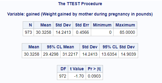
To do:
- Find the observed sample statistic, \(\bar{x}\) (30.3)
- Find the observed standard deviation, \(s\) (14.2)
- Find the confidence interval for the mean (27.4, 31.2)
- Find the estimated t-statistic (-1.70) and the associated p-value (0.090)
Values may differ slightly here from above based on the fact that we rounded a few of the quantities above. The conclusions remain the same.
You have successfully completed this tutorial.